This week Things has a very slight Hallowe’en theme.
Puzzle
This is one where you should gather some people around the monitor and see who can do best: guess the cartoon (or CG) character from their eyes (mouse over the eyes to see the character outline that should tell you if you’re right).
And yes, it is pretty difficult – I only got 6, and I watch a lot of animation!
Video
Here’s a video that begs the question: is the cat playing the game, or just acting out of blind instinct?
http://www.youtube.com/watch?v=QrlTijuhVOA
To which the answer is to have a big argument about the definitions being used before concluding that you can’t tell.
Quote
In the wonderfully stylised animation The Secret of Kells, I heard the line “One beetle recognises another” and wondered if it was some kind of proverb. It turns out that it is, and actually – obviously – there are a whole bunch of Irish Proverbs, which in translated form become alternately profound, banal or hilarious, just as I imagine English proverbs must seem if you haven’t grown up with them. Here’s a list of them on Wikiquote, and here are a few of my favourites, for unstated reasons:
“Every beginning is weak.”
“Time is a good story teller.”
“A lamb becomes a sheep with distance…”
“The quiet are guilty”
Comic
The Enigma of Amigara Fault is a horror comic that impressed me with its unconventional approach. It’s 32 pages, and originally in Japanese so you have to read the panels right to left. But if you want a comic that will freak you out for Hallowe’en, it’s worth it. Unless you’re particularly claustrophobic, in which case you should probably steer clear of it entirely.
Answer – Malady X
In Things 111 I asked what the probability of having Malady X is if a randomly administered 99%-accurate test for it comes back positive. As Phil and Thomas noted, you can’t actually answer from this information alone: you also have to know what the probability of a random person actually having Malady X is. A lot of people don’t have an intuition for this fact. I’m going to attempt to explain ways to apprehend that hand-wavingly, mathematically, and visually.
Argument from hand waving and examples:
Imagine the probability of having Malady X is 0% – nobody has it. In this case, it’s certain that getting a positive result means you were simply in the 1% of cases where the test comes back incorrect.
Conversely if the probability of having it is 100% – everybody has it – then you must be in the 99% of cases where it is accurate. In this way, it’s clear the underlying probability influences the chances that the test is correct!
We might worry that these extremes somehow break the puzzle, so let’s imagine less extreme alternatives. Imagine 1,000 people are tested. If 50% (500) really have Malady X, on average we expect the test to come back positive for 99% of them (495) and also for 1% of the 500 that don’t have it (5). In this situation, 495 out of the 500 people for whom the test was positive actually have the disease – 99%.
Alternatively, if 1 person (or 0.1%) out of the 1,000 has the disease, they’re very likely to be correctly diagnosed, and we expect roughly 10 of the other 999 to get a positive result. In this case 1 out of 11 people with a positive result actually have Malady X – fewer than 10%. So clearly the underlying incidence level matters.
Argument from maths:
There are two probabilities at work: the chance the test is correct (99%) and the chance of anyone having Malady X (unknown – let’s call it X%). When you combine probabilities you multiply them, so for example the chance of anyone actually having Malady X AND getting a postive result is 99% times X%.
If someone gets a positive result and that’s all we know, we reason as follows:
A = Probability someone has Malady X and tests positive = X% times 99% times
B = Probability someone does not have Malady X but still tests positive = (100% – X%) times 1%
If you test positive, the chance you actually have it is C = A / (A+B). But if you haven’t studied probability carefully, I’m not sure you could infer this, which is why I like to come up with other ways of getting a feel for the correct answer.
Argument from visualisation:
Since there are two probabilities in question, and we combine probabilities by multiplying, this naturally suggests a visualisation where probability is represented by rectangular area (since area is calculated by multiplying height by breadth).
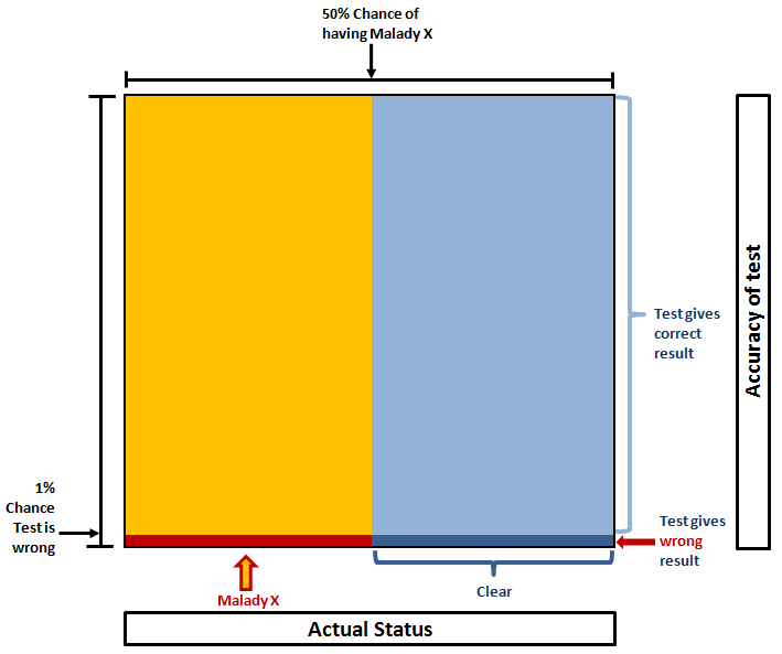
For example, if we imagine the actual incidence rate of Malady X is 50%, the picture would look like this (click for big):
If the test result is positive, you either have it and the result is correct (big yellow area) or you don’t have it but the test was incorrect (small dark blue area). The chance of you actually having Malady X is equal to the proportion of those combined areas that is yellow. In this case:
Yellow = 99% x 50% = 49.5%
Dark blue = 1% * 50% = 0.5%
Probability you have it = Proportion that is yellow = 49.5% / (49.5% + 0.5%) = 99%.
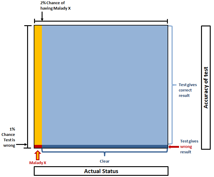
Alternatively if the incidence rate is, say, 2%, it looks like this:
Here we see the yellow and dark blue areas are very similar, so the chance of you being one or the other is much more even. In fact, it’s:
Yellow = 99% x 2% = 1.98%
Dark blue = 1% x 98% = 0.98%
Probability you have it = Proportion that is yellow = 1.98% / (1.98% + 0.98%) = 67% (ish).
As Peter Donnelly shows in this TED talk, this actually has some severe ramifications, because when the probability of the thing being tested for is extremely low, it becomes overwhelmingly likely that a positive result is false, but people intuitively feel that a 99% accurate test should be correct 99% of the time.
Thomas also noted:
If anyone is interested in playing around with the probabilities (even if you’re not familiar with the maths), I recommend GeNIe:
http://genie.sis.pitt.edu/
It lets you create networks of dependencies, set evidence and work out probabilities in problems just like these.
-Transmission finally ends

